![]()
1. Verification with analytical source
1.1. Install KDSource
[ ]:
#
# Executing this cell you will install KDSource
# in this instance of the Google Colaboratory virtual machine.
# The process takes about 1 minutes.
#

def install_kdsource():
  #
  # Clone source code from Github, make and install
  #

  import os

  if not os.path.isdir('/content'):
    print("This function installs KDSource in a Google Colaboratory instance.")
    print("To install locally follow instructions in documentation:")
    print("link/to/docs?")
    return

  %cd -q /content
  print("Obtaining KDSource source code from Github...")
  !git --no-pager clone --recurse-submodules https://$username:$password@github.com/inti-abbate/KDSource &> /dev/null
  %cd -q KDSource
  !git --no-pager checkout master &> /dev/null
  !mkdir build
  %cd -q build
  print("Running cmake...")
  !cmake .. -DCMAKE_INSTALL_PREFIX=/usr/local/KDSource &> /dev/null
  print("Running make install...")
  !make install &> /dev/null
  print("Installing Python API...")
  %cd -q ../python
  !pip install . &> /dev/null

  os.environ['PATH'] += ":/usr/local/KDSource/bin"

  %cd -q /content

from time import time
t1 = time()
install_kdsource()
t2 = time()
print("Installed KDSource in {:.2f} minutes".format((t2-t1)/60.0))
1.2. Generate synthetic data
A particle list will be generated with the following joint distribution:
Being \(u=log(E_0/E)\) the lethargy, \((x,y)\) the 2D position (\(z\) is fixed at 0), and \(\mu=cos(\theta),\phi\) the polar coordinates, so that \(\hat{\Omega}=(d_x,d_y,d_z)=(sin(\theta)cos(\phi),sin(\theta)sin(\phi),cos(\theta))\) is the direction unit-vector.
This means that there are two “clusters” of particles, each one with a characteristic energy and x distribution, implying that this variables are correlated. The other variables have a separated density distribution.
The specific distributions for each variable are described as follows:
Energy: Normal distribution for lethargy, for each cluster:
\[f_{U,i}(u)=\frac{1}{\sigma_u\sqrt{2\pi}}exp\left(-\frac{(u-\mu_{u,i})^2}{2\sigma_u^2}\right),\ i=1,2\]Position: Normal distribution for x, for each cluster. Normal distribution around 0 for y. Fixed z = 0:
\[f_{x,i}(x)=\frac{1}{\sigma_x\sqrt{2\pi}}exp\left(-\frac{(x-\mu_{x,i})^2}{2\sigma_x^2}\right),\ i=1,2,\ f_y(y)=\frac{1}{\sigma_y\sqrt{2\pi}}exp\left(-\frac{y^2}{2\sigma_y^2}\right)\]Direction: “Cosine distribution”, uniform in φ:
\[f_{\mu}(\mu)=2\mu,\ \mu>0,\ f_{\phi}(\phi)=\frac{1}{2\pi}\]Weight: Normal distribution around 1.
\[f(w)=\frac{1}{\sigma_w\sqrt{2\pi}}exp\left(-\frac{(w-1)^2}{2\sigma_w^2}\right)\]with σw small enough so that w is always greater than 0.
[1]:
import os
import numpy as np
import kdsource as kds
import mcpl

N = int(1E5) # Size of particle list

pt = "n"     # Particle type: neutron

# Energy
E0 = 10.0
sigma_u = 1
mu_u_1 = 5
mu_u_2 = 9
us_1 = np.random.normal(mu_u_1, sigma_u, (int(N/2),1))
us_2 = np.random.normal(mu_u_2, sigma_u, (int(N/2),1))
us = np.concatenate((us_1, us_2), axis=0)
Es = E0 * np.exp(-us)
# Position
sigma_x = sigma_y = 10
mu_x_1 = sigma_x
mu_x_2 = -sigma_x
poss_1 = np.random.normal([mu_x_1,0,0], [sigma_x,sigma_y,0], (int(N/2),3))
poss_2 = np.random.normal([mu_x_2,0,0], [sigma_x,sigma_y,0], (int(N/2),3))
poss = np.concatenate((poss_1, poss_2), axis=0)
# Direction
mus = np.sqrt(np.random.uniform(0,1,N))
phis = np.random.uniform(-np.pi,np.pi,N)
dxs = np.sqrt(1-mus**2) * np.cos(phis)
dys = np.sqrt(1-mus**2) * np.sin(phis)
dzs = mus
dirs = np.stack((dxs,dys,dzs), axis=1)
# Time
ts = np.zeros((N,1))
# Stack energies, positions, directions and times
parts = np.concatenate((Es,poss,dirs,ts), axis=1)
np.random.shuffle(parts)

# Weights
sigma_w = 0.1
ws = np.random.normal(1, sigma_w, N)

ssvfile = "samples.ssv"
kds.savessv(pt, parts, ws, ssvfile)
!ssv2mcpl $ssvfile samples
samples = "samples.mcpl.gz"
Writing particles into SSV file...
Done. All particles written into samples.ssv
ssv_open_file: Opened file "samples.ssv":
MCPL: Attempting to compress file samples.mcpl with gzip
MCPL: Succesfully compressed file into samples.mcpl.gz
Created samples.mcpl.gz
1.3. Create and optimize KDSource
1.3.1. Create KDSource
[2]:
# PList: wrapper for MCPL file
plist = kds.PList(samples)
# Geometry: define metrics for variables
geom = kds.Geometry([kds.geom.Lethargy(E0),
                     kds.geom.SurfXY(),
                     kds.geom.Isotrop()])
# Create KDSource
s = kds.KDSource(plist, geom)
Using existing file samples.mcpl.gz
sum_weights = 99977.3360118866
p2 = 100956.6509826754
N = 100000
N_eff = 99007.52074025258
1.3.2. Optimize bandwidth
[3]:
# Give a little more importance to energy
var_importance = [3,1,1,1,1,1]

parts,ws = s.plist.get(N=-1)
scaling = s.geom.std(parts=parts)
scaling /= var_importance
[4]:
# Number of particles to use for optimization.
# A large number (1E5 or more) gives better bandwidths, but takes longer to
# compute.
N = 1E5
Choose one of the available bandwidth optimization methods. Recommended method is Method 3 (adaptive MLCV)
[5]:
# Method 1: Silverman's Rule: Simple and fast method.
# BW is chosen based on only on the number of particles, and dimension of
# geometry.

s.bw_method = "silv"
s.fit(N, scaling=scaling)
Using 100000 particles for fit.
Calculating bw ...
Done
Optimal bw (silv) = [[0.2195508  4.18463626 2.949225   0.13930225 0.13930225 0.13930225]]
[6]:
# Method 2: Non-adaptive Maximum Likelihood Cross-Validation:
# Creates a grid of non-adaptive bandwidths and evaluates the
# cross-validation scores on each one, which is an indicator of the
# quality of the estimation. Selects the bandwidth that optimizes
# CV score.

s.bw_method = "mlcv"
seed = None # Default: Use the Silverman's Rule as seed
grid = np.logspace(-0.1,0.1,10)

N_cv = int(1E4) # Use a smaller N to reduce computation times
s.fit(N_cv, scaling=scaling, seed=seed, grid=grid)

bw = s.kde.bw
dim = s.geom.dim
bw *= kds.kde.bw_silv(dim,N)/kds.kde.bw_silv(dim,N_cv) # Apply Silverman factor
s = kds.KDSource(plist, geom, bw=bw) # Create new KDSource with adapted BW
s.fit(N=N, scaling=scaling)
Using 10000 particles for fit.
Calculating bw ...
[Parallel(n_jobs=-1)]: Using backend LokyBackend with 8 concurrent workers.
[Parallel(n_jobs=-1)]: Done   3 out of  10 | elapsed:    8.3s remaining:   19.3s
[Parallel(n_jobs=-1)]: Done   5 out of  10 | elapsed:    8.7s remaining:    8.7s
[Parallel(n_jobs=-1)]: Done   7 out of  10 | elapsed:    9.1s remaining:    3.9s
[Parallel(n_jobs=-1)]: Done  10 out of  10 | elapsed:   12.7s finished
Done
Optimal bw (mlcv) = [[0.25597761 4.87893091 3.43854617 0.16241461 0.16241461 0.16241461]]
Using 100000 particles for fit.
[7]:
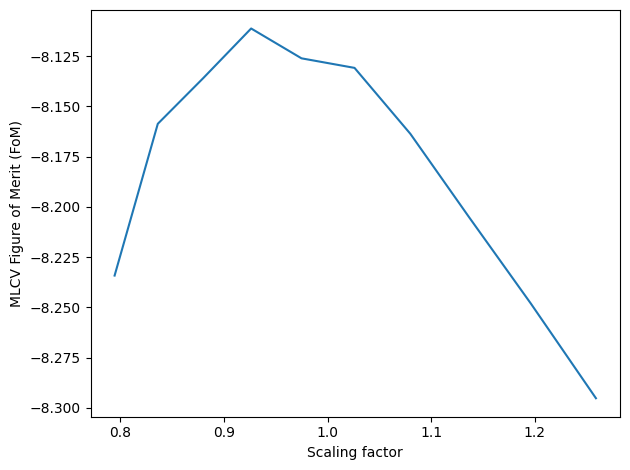
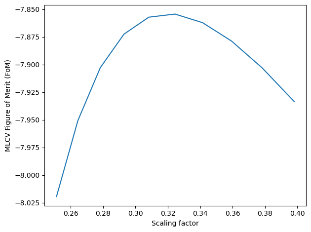
# Method 3: Adaptive Maximum Likelihood Cross-Validation:
# Creates a grid of adaptive bandwidths and evaluates the
# cross-validation scores on each one, which is an indicator of the
# quality of the estimation. Selects the bandwidth that optimizes
# CV score.
# kNN is used to generate the seed adaptive bandwidth.

# kNN bandwidth
s.bw_method = "knn"
batch_size = 10000 # Batch size for KNN search
k = 10             # Numer of neighbors per batch
s.fit(N, scaling=scaling, batch_size=batch_size, k=k)
bw_knn = s.kde.bw

# MLCV optimization of previously calculated kNN bandwidth
s.bw_method = "mlcv"
N_cv = int(1E4)   # Use a smaller N to reduce computation times
seed = bw_knn[:N_cv] # Use kNN BW as seed (first N elements)
grid = np.logspace(-0.6,-0.4,10)
s.fit(N_cv, scaling=scaling, seed=seed, grid=grid)
bw_cv = s.kde.bw

# Extend MLCV optimization to full KNN BW
bw_knn_cv = bw_knn * bw_cv[0]/bw_knn[0] # Apply MLCV factor
dim = s.geom.dim
bw_knn_cv *= kds.kde.bw_silv(dim,len(bw_knn))/kds.kde.bw_silv(dim,len(bw_cv)) # Apply Silverman factor
s = kds.KDSource(plist, geom, bw=bw_knn_cv) # Create new KDSource with full BW
s.fit(N=N, scaling=scaling)
Using 100000 particles for fit.
Calculating bw ...
Using k = 10 neighbors per batch (batch_size = 10000)
Correction factor: f_k = k_float / k = 1.0
Effective total neighbors: K_eff = 100.0
batch = 1 / 10
batch = 2 / 10
batch = 3 / 10
batch = 4 / 10
batch = 5 / 10
batch = 6 / 10
batch = 7 / 10
batch = 8 / 10
batch = 9 / 10
batch = 10 / 10
Done
Optimal bw (knn) = [[ 0.58540492 11.15781225  7.86374173  0.37143213  0.37143213  0.37143213]
 [ 0.7103917  13.54005908  9.54268858  0.45073469  0.45073469  0.45073469]
 [ 0.7108049  13.5479347   9.54823912  0.45099686  0.45099686  0.45099686]
 ...
 [ 0.74495647 14.19886324 10.00699697  0.47266561  0.47266561  0.47266561]
 [ 0.45203682  8.61581749  6.0722086   0.28681173  0.28681173  0.28681173]
 [ 0.66823837 12.7366171   8.97644315  0.42398893  0.42398893  0.42398893]]
Using 10000 particles for fit.
Calculating bw ...
[Parallel(n_jobs=-1)]: Using backend LokyBackend with 8 concurrent workers.
[Parallel(n_jobs=-1)]: Done   3 out of  10 | elapsed:   19.6s remaining:   45.8s
[Parallel(n_jobs=-1)]: Done   5 out of  10 | elapsed:   22.9s remaining:   22.9s
[Parallel(n_jobs=-1)]: Done   7 out of  10 | elapsed:   26.1s remaining:   11.2s
[Parallel(n_jobs=-1)]: Done  10 out of  10 | elapsed:   37.2s finished
Done
Optimal bw (mlcv) = [[0.18991859 3.61984655 2.5511756  0.12050098 0.12050098 0.12050098]
 [0.23046713 4.39270128 3.09586392 0.14622852 0.14622852 0.14622852]
 [0.23060118 4.39525631 3.09766464 0.14631358 0.14631358 0.14631358]
 ...
 [0.15920815 3.03450579 2.13864235 0.10101559 0.10101559 0.10101559]
 [0.27045949 5.15495528 3.63308112 0.17160318 0.17160318 0.17160318]
 [0.19201307 3.65976728 2.57931072 0.1218299  0.1218299  0.1218299 ]]
Using 100000 particles for fit.
1.4. Resample
[8]:
xmlfile = "source.xml"
s.save(xmlfile) # Save KDSource to XML file

N_resampled = 1E6 # Number of particles to generate with virtual KDE source
if os.name == 'posix':
    !kdtool resample "$xmlfile" -o "resampled" -n $N_resampled
if os.name == 'nt': # kdtool still not implemented in Windows
    !kdtool-resample "$xmlfile" -o "resampled" -n $N_resampled
resampled = "resampled.mcpl.gz"
Bandwidth file: samples_bws
Successfully saved parameters file source.xml
Reading xmlfile source.xml...
Done.
Resampling...
MCPL: Attempting to compress file resampled.mcpl with gzip
MCPL: Succesfully compressed file into resampled.mcpl.gz
Successfully sampled 1000000 particles.
A new MCPL file has been created, named “resampled.mcpl.gz”, with particles generated from the KDE-based distribution.
1.5. Create plots
The following plots compare the analytic distributions with the KDSource kernel density estimations, and the histograms of the resampled data, to verify that they match.
Comparison is performed both visually and quantitatively, based on the Kullback-Leibler divergence.
[9]:
import matplotlib.pyplot as plt
[10]:
# KL divergence
# Notice that p and q should be evaluated in a regular (linear) grid
def kl_divergence(p, q):
  return np.sum(np.where(p != 0, p * np.log(p / q), 0))

# Histogram of MCPL particle list
def mcpl_hist(mcplfile, var, bins, part0=None, part1=None, **kwargs):
  pl = mcpl.MCPLFile(mcplfile)
  hist = np.zeros(len(bins)-1)
  I = 0
  for pb in pl.particle_blocks:
    parts = np.stack((pb.ekin,pb.x,pb.y,pb.z,pb.ux,pb.uy,pb.uz), axis=1)
    mask1 = np.ones(len(parts), dtype=bool)
    if part0 is not None:
      mask1 = np.logical_and.reduce(part0 <= parts, axis=1)
    mask2 = np.ones(len(parts), dtype=bool)
    if part1 is not None:
      mask2 = np.logical_and.reduce(parts <= part1, axis=1)
    mask = np.logical_and(mask1, mask2)
    data = parts[mask][:,var]
    hist += np.histogram(data, bins=bins, weights=pb.weight[mask], **kwargs)[0]
    I += np.sum(pb.weight)
  hist /= I
  hist /= (bins[1:]-bins[:-1])
  return hist

# Simple power law
def powerlaw(x, C, a):
    return C * x**a
1.5.1. Energy plots
[11]:
EE = np.logspace(-4,0,50)

# Analytic distributions
uu = s.geom.ms[0].transform(EE)
pdf_1 = 0.5 * 1/EE*np.exp(-(uu-mu_u_1)**2/(2*sigma_u**2))/(sigma_u*np.sqrt(2*np.pi))
pdf_2 = 0.5 * 1/EE*np.exp(-(uu-mu_u_2)**2/(2*sigma_u**2))/(sigma_u*np.sqrt(2*np.pi))
f = 0.1587 # Integral of normal distribution for x-mu>std
[12]:
# Plot energy distribution

fig,scores = s.plot_E(EE, label="KDE")

hist = mcpl_hist(resampled, 0, EE)
widths = (EE[1:]-EE[:-1])
plt.bar(EE[:-1], hist, width=widths, align="edge", linewidth=.5, ec="k",
        fc="g", alpha=.7, label="Resampled")

plt.plot(EE, pdf_1+pdf_2, 'xr', zorder=1, label="Analytic")

plt.legend()
plt.tight_layout()
plt.savefig('E-true-KDE-hist.pdf')
plt.show()
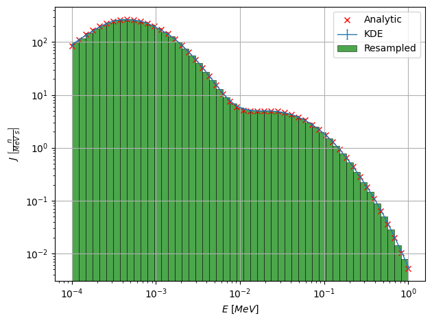
It can be seen that the KDE successfully estimates the original distribution.
[13]:
# Plot reduction of KL divergence with growing N

# KL divergence is computed between lethargy distributions
# because energy grid is logarithmic (linear in lethargy)

s.bw_method = None
KLDs = []
n_vals = np.logspace(2,5,7).astype("int")
dim = s.geom.dim
bw = s.kde.bw
for n in n_vals:
  s.fit(N=n, scaling=scaling)
  s.kde.bw = bw * kds.kde.bw_silv(dim,n)/kds.kde.bw_silv(dim,N)
  fig,[score,err] = s.plot_E(EE, label=f"N = {n}")
  f_u = (pdf_1+pdf_2) * EE # Analytic lethargy distribution
  KDE_u = score * EE       # KDE lethargy distribution
  KLDs.append(kl_divergence(f_u, KDE_u))
plt.clf()

print((KLDs[-1]-KLDs[-3]) / (KLDs[-3]-KLDs[-5]))
print((KLDs[-1]-KLDs[-3]) / (KLDs[2]-KLDs[0]))

plt.plot(n_vals, KLDs, 'o-')
plt.xlabel('Number of particles')
plt.ylabel('$D_{KL}(\,\hat{f}\,||\,f\,)$')
plt.title('Kullback-Leibler Divergence')
plt.xscale('log')
plt.yscale('log')
plt.grid()
plt.savefig('convergence-KLD.pdf', bbox_inches='tight')
plt.show()
Using 100 particles for fit.
Using 316 particles for fit.
Using 1000 particles for fit.
Using 3162 particles for fit.
Using 10000 particles for fit.
Using 31622 particles for fit.
Using 100000 particles for fit.
0.09434937613872689
0.008635154007072378
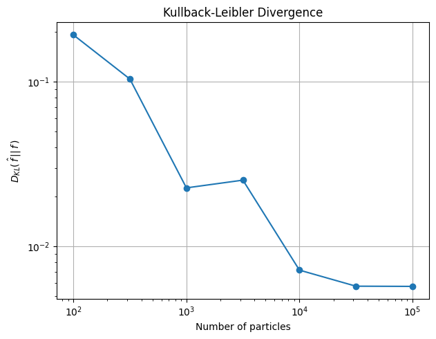
It can be seen how the KL divergence between the true and estimated distribution decreases with the number of particles.
[14]:
# Plot correlation with x

# Vectors to separate x<0 and x>0
# Vec: [u, x,y, dx,dy,dz]
vec0 = [-np.inf,0,-np.inf,-1,-1,-1]
vec1 = [np.inf,0,np.inf,1,1,1]
# Part: [E, x,y,z, dx,dy,dz]
part0 = [0,0,-np.inf,-np.inf,-1,-1,-1]
part1 = [np.inf,0,np.inf,np.inf,1,1,1]

# Plot only particles with x > 0
fig,scores = s.plot_E(EE, vec0=vec0, label="x>0, KDE")
plt.gca().lines[0].set_linewidth(1.5)
plt.plot(EE, (1-f)*pdf_1+f*pdf_2, 'x', linewidth=1.5, label="x>0, Analytic")

# Plot only particles with x < 0
fig,scores = s.plot_E(EE, vec1=vec1, label="x<0, KDE")
plt.gca().lines[0].set_linewidth(1.5)
plt.plot(EE, f*pdf_1+(1-f)*pdf_2, 'x', linewidth=1.5, label="x<0, Analytic")

plt.grid()
plt.legend()
plt.tight_layout()
plt.savefig("E-correl.pdf")
plt.show()
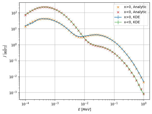
Since energy and x are correlationated, restricting the x values affects the energy distribution.
Since the two energy-x clusters overlap in x, particles with x>0 are composed by a big fraction of the cluster with μx>0, but also a small fraction of the other cluster. The energy peaks are thus modified with the respective factors, as can be seen in the plot. The analogous effect happens for particles with x<0.
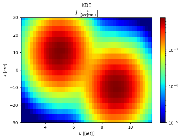
[15]:
# Lethargy-x 2D plot

xx = np.linspace(-30,30,20)

fig,scores = s.plot2D_integr(["u","x"], [uu,xx], scale="log")

plt.clim(vmin=1e-5)
plt.tight_layout()
plt.savefig("u-x.pdf")
plt.show()
1.5.2. Position plots
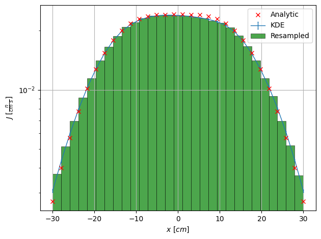
[16]:
# Plot x distribution

xx = np.linspace(-30,30,30)
pdf_1 = 0.5 * np.exp(-((xx-mu_x_1)/sigma_x)**2/2)/(sigma_x*np.sqrt(2*np.pi))
pdf_2 = 0.5 * np.exp(-((xx-mu_x_2)/sigma_x)**2/2)/(sigma_x*np.sqrt(2*np.pi))

fig,scores = s.plot_integr("x", xx)

hist = mcpl_hist(resampled, 1, xx)
widths = (xx[1:]-xx[:-1])
plt.bar(xx[:-1], hist, width=widths, align="edge", linewidth=.5, ec="k",
        fc="g", alpha=.7, label="Resampled")

plt.plot(xx, pdf_1+pdf_2, 'xr', zorder=3, label="Analytic")

plt.legend()
plt.tight_layout()
plt.savefig("x.pdf")
plt.show()
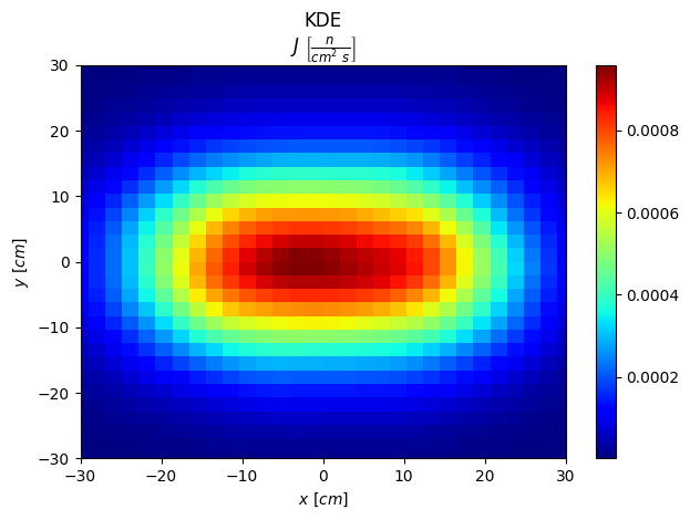
[17]:
# Plot xy distribution

xx = np.linspace(-30,30,30)
yy = np.linspace(-30,30,30)
fig,scores = s.plot2D_integr(["x","y"], [xx,yy])
plt.tight_layout()
plt.show()
1.5.3. Direction plots
[20]:
# Plot dz distribution

ddz = np.linspace(0,1,30)
pdf = 2 * ddz

fig,[scores,errs] = s.plot_integr("dz", ddz, yscale="linear")

hist = mcpl_hist(resampled, 6, ddz)
hist = np.concatenate((hist, hist[-1:]))
plt.plot(ddz, hist, ds='steps-post', label="Resampled")

plt.plot(ddz, pdf, 'x', zorder=3, label="Analytic")

fig,[scores,errs] = s.plot_integr("dz", ddz, vec0=vec0, yscale="linear", label="x>0, KDE")

hist = mcpl_hist(resampled, 6, ddz, part0=part0)
hist = np.concatenate((hist, hist[-1:]))
plt.plot(ddz, hist, ds='steps-post', label="x>0, Resampled")

plt.plot(ddz, 0.5*pdf, 'x', zorder=3, label="x>0, Analytic")

plt.ylim(bottom=0)
plt.grid()
plt.legend()
plt.tight_layout()
plt.savefig("mu-x.pdf")
plt.show()
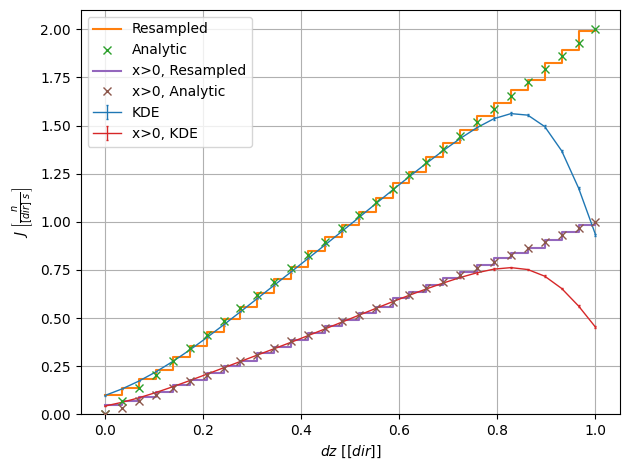
Since mu is not correlated with x, its distribution for x>0 is the same (linear), but with half the intensity.
Besides, although the Python KDE fails to match the analytic distribution near dz=1, due to border effects, the resampled data do match it. This is because the sampling algorithms take into account the nature of the direction vector.
[19]:
# Plot dx-dy distribution

ddx = np.linspace(-1,1,30)
ddy = np.linspace(-1,1,30)

fig,scores = s.plot2D_integr(["dx","dy"], [ddx,ddy], scale="linear")

plt.gca().set_aspect(1)
plt.tight_layout()
plt.savefig("x-y.pdf")
plt.show()
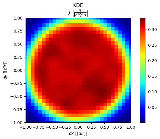
For a cosine distribution, the density projected in the dx-dy plane is uniform.
[ ]: